Understanding Deep Learning: From Basics to Neural Networks
Imagine teaching a computer to see the world like we do - that’s what Deep Learning does! It’s like giving a computer a super-powered brain that can learn to recognize cats in photos, understand human speech, or even predict tomorrow’s weather. If you’re familiar with basic machine learning concepts like training data and models, this guide will show you how Deep Learning takes these ideas to the next level using neural networks.
What is Deep Learning?
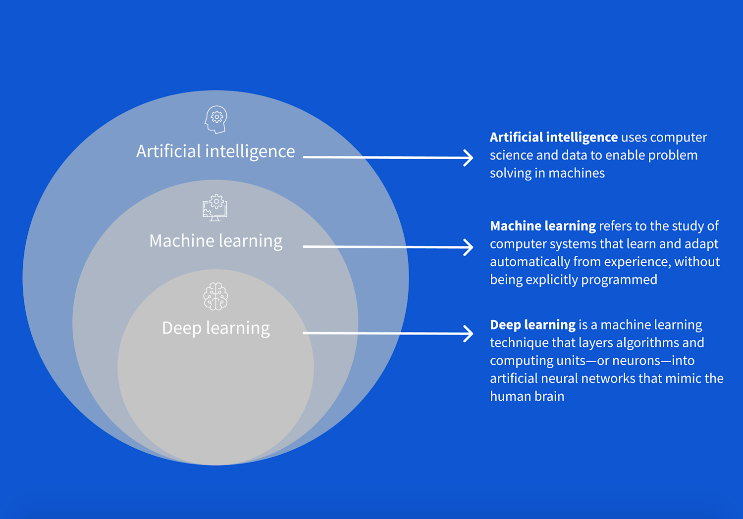
Deep Learning (DL) is a specialized subset of machine learning that uses artificial neural networks with multiple layers (hence “deep”) to progressively extract higher-level features from raw input. This hierarchical learning process mimics how the human brain processes information.

Some foundational concepts to keep in mind:
- Machine Learning is teaching computers to learn from examples, like showing a child many pictures of cats until they can recognize new cats they’ve never seen before
- Neural Networks are computer systems inspired by human brain cells (neurons) that work together to solve problems. We’ll dive into how they work in more detail later.
- Deep Learning happens when we stack many layers of these artificial neurons to tackle complex tasks
Think of it like this: if traditional programming is like giving a computer step-by-step instructions to bake a cake, Deep Learning is more like showing the computer thousands of successful cakes and letting it figure out the recipe on its own!
How Deep Learning Works
Feature Hierarchy
- First layers detect basic features (edges, colors, textures)
- Middle layers combine these to identify patterns (shapes, parts)
- Deep layers recognize complex concepts (objects, scenes, contexts)
Learning Process
- Automatic feature extraction through multiple transformations
- Layer-by-layer representation learning
- End-to-end optimization of the entire pipeline
Real-World Applications
Computer Vision
- Object detection and recognition
- Facial recognition systems
- Medical image analysis
- Autonomous vehicle perception
Natural Language Processing
- Language translation
- Sentiment analysis
- Text generation
- Speech recognition
Time Series Analysis
- Stock market prediction
- Weather forecasting
- Demand prediction
- Anomaly detection
Deep Learning vs Traditional Machine Learning
Traditional machine learning and deep learning differ in several key aspects:
| Traditional ML | Deep Learning |
|---|---|
| Requires manual feature engineering | Automatically learns features |
| Works well with smaller datasets | Needs large amounts of data |
| More interpretable | Often acts as a “black box” |
| Less computational resources | Requires significant computing power |
| Linear and structured data | Handles unstructured data well |
Key Differences in Detail
Feature Engineering
- Traditional ML requires domain expertise to create features
- Deep Learning automatically learns relevant features
- Example: In image recognition
# Traditional ML approach
def extract_features(image):
    edges = detect_edges(image)
    textures = compute_textures(image)
    colors = extract_color_histogram(image)
    return np.concatenate([edges, textures, colors])

# Deep Learning approach
model = tf.keras.applications.ResNet50(weights='imagenet')
# Features are learned automatically through training
Scalability with Data
- Traditional ML performance plateaus with more data
- Deep Learning continues to improve with more data
- Computational requirements scale differently
Model Complexity
- Traditional ML models have fewer parameters
- Deep Learning models can have millions/billions of parameters
- Example architecture comparison:
# Traditional ML (Random Forest)
rf_model = RandomForestClassifier(n_estimators=100)

# Deep Learning (Complex CNN)
dl_model = tf.keras.Sequential([
    layers.Conv2D(64, 3, activation='relu'),
    layers.MaxPooling2D(),
    layers.Conv2D(128, 3, activation='relu'),
    layers.MaxPooling2D(),
    layers.Conv2D(256, 3, activation='relu'),
    layers.Flatten(),
    layers.Dense(512, activation='relu'),
    layers.Dense(num_classes, activation='softmax')
])
Neural Networks: The Building Blocks
Think of a neural network like a complex assembly line in a factory, where each station (layer) processes materials (data) in specific ways. Let’s break down the main components:
1. Layers: The Assembly Line Stations
Input Layer
- Acts as the data reception desk of our neural network
- Formats and standardizes incoming data based on the type of input:
- Images: Resize to fixed dimensions (e.g., 224x224 pixels), normalize pixel values (0-1)
- Text: Convert words to numbers (word embeddings or one-hot encoding)
- Numerical: Scale features (normalization or standardization)
- Categorical: Convert to one-hot vectors
- Time Series: Create sequences of fixed length
Here are some common examples:
# Image data preparation
def prepare_image(image_path):
    image = tf.keras.preprocessing.image.load_img(
        image_path,
        target_size=(224, 224)  # Standard size for many models
    )
    return tf.keras.preprocessing.image.img_to_array(image) / 255.0  # Normalize to 0-1

# Text data preparation
def prepare_text(text):
    tokenizer = tf.keras.preprocessing.text.Tokenizer()
    tokenizer.fit_on_texts([text])
    return tokenizer.texts_to_sequences([text])[0]

# Numerical data preparation
def prepare_numerical(data):
    scaler = StandardScaler()  # or MinMaxScaler()
    return scaler.fit_transform(data)

# Categorical data preparation
def prepare_categorical(category):
    encoder = OneHotEncoder()
    return encoder.fit_transform([[category]]).toarray()

# Time series preparation
def prepare_timeseries(data, sequence_length=10):
    sequences = []
    for i in range(len(data) - sequence_length):
        sequences.append(data[i:i + sequence_length])
    return np.array(sequences)
Each type of input requires different preprocessing to work effectively with neural networks. The key is to convert all inputs into numerical formats that the network can process.
Hidden Layers
- The “thinking” parts of the network where the magic happens
- Multiple layers work together to understand complex patterns
- Each layer specializes in different levels of abstraction
- Example: In a face recognition system
- First hidden layer: Detects edges and basic shapes
- Second hidden layer: Combines edges into features (eyes, nose)
- Third hidden layer: Assembles features into face patterns
Output Layer
- The final decision-making layer
- Shape depends on your task:
- Single node for yes/no decisions (Is this a cat?)
- Multiple nodes for multiple choices (Which digit is this: 0-9?)
# Example output layer configurations
# Binary classification (yes/no)
output_layer = layers.Dense(1, activation='sigmoid')

# Multi-class classification (multiple choices)
output_layer = layers.Dense(10, activation='softmax')

2. Neurons: The Workers in Our Factory
Each neuron is like a tiny calculator that:
Processes Inputs
- Receives information from previous layer neurons
- Weighs each input’s importance (like judges in a competition)
- Example: A neuron looking at a cat image might give high importance to ear shapes
Performs Calculations
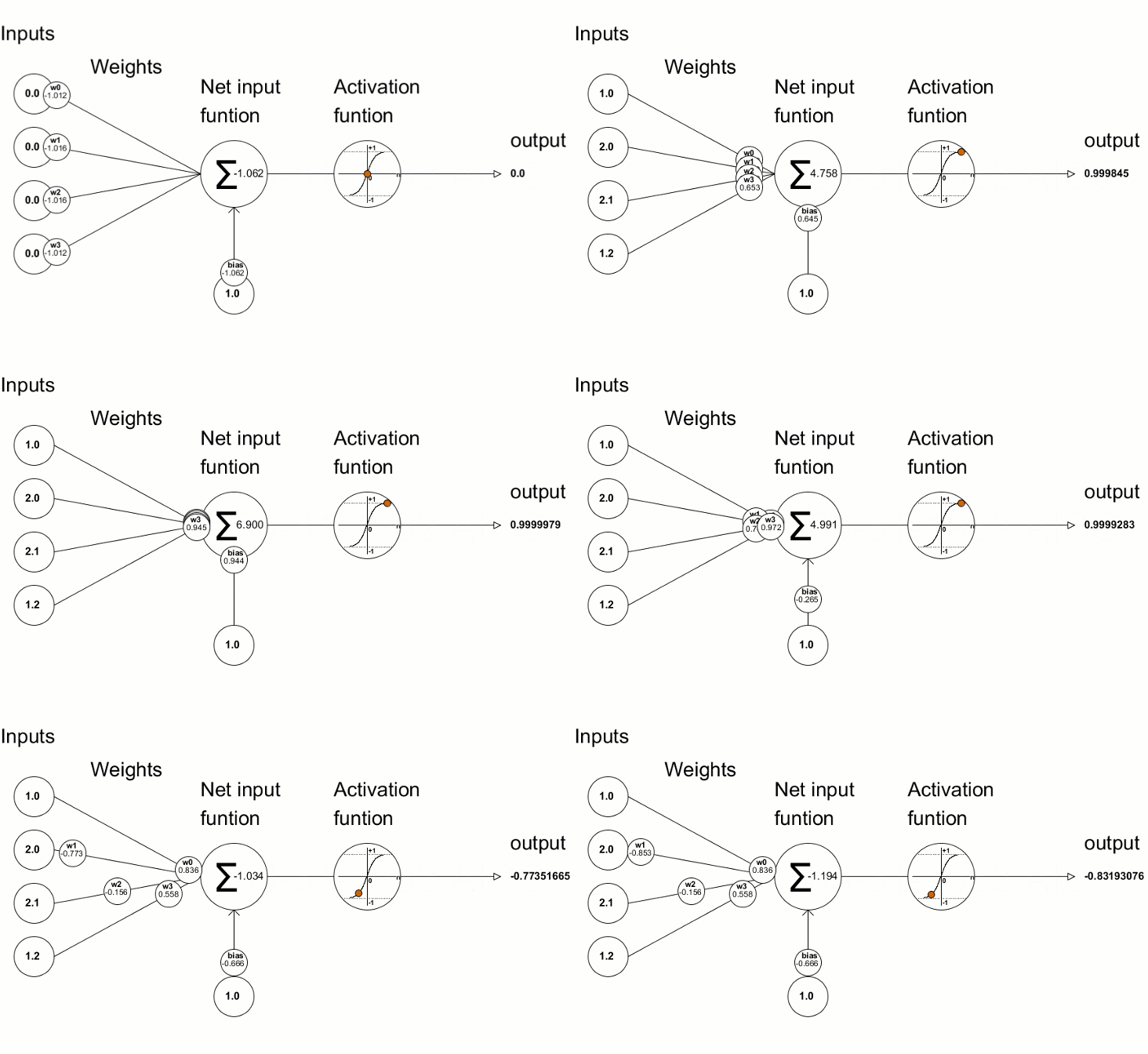
Each neuron is just basically a function that takes the inputs, weights and bias and applies the activation function to it. We can imagine it similar to regression, where we have a function that takes the inputs and weights and bias and applies the activation function to it. The difference is that in neural networks, we perform this operation in multiple neurons / units and layers.
An overview of neural network calculation is shown below:

# Simplified example of what happens inside a neuron
def neuron_calculation(inputs, weights, bias):
    # Step 1: Multiply each input by its weight
    weighted_sum = sum(input * weight for input, weight in zip(inputs, weights))

    # Step 2: Add bias (like a base score)
    total = weighted_sum + bias

    # Step 3: Apply activation function (decision maker)
    output = max(0, total)  # Using ReLU activation
    return output
Makes Decisions
- Uses activation functions to decide whether to “fire” (activate)
- Common activation functions and their real-world analogies:
- ReLU: filters out negative values (lets in positive values, stops negatives)
- Sigmoid: converts numbers to 0-1 scale
- Tanh: converts numbers to -1 to +1 scale
3. Connections: The Communication Network
Weights
- Like the importance scores in a relationship
- Start random and get adjusted during training
- Example: In a cat detector
# Visualizing weight importance
def print_weight_importance(weights):
    """Shows which features the model thinks are important"""
    for i, w in enumerate(weights):
        importance = abs(w)
        print(f"Feature {i}: {'#' * int(importance * 10)}")
Bias Terms
- Act like a threshold for activation
- Help neurons make better decisions
- Real-world analogy: Like your personal preference before reviewing evidence
- If you love cats, you might be biased to see cats everywhere
- The bias term helps balance this out
Activation Functions in Action
Why do neural networks need activation functions? Without them, neural networks would just be a series of linear transformations, no matter how many layers we add! Activation functions introduce non-linearity, allowing networks to learn complex patterns and relationships in data.
Think of it this way: if you’re trying to draw a curved line using only straight lines, you’ll need many short straight segments to approximate the curve. Activation functions let our network create those “curves” naturally.

Here are the most common activation functions and their use cases:
# Common activation functions explained
import numpy as np

def relu(x):
    """
    The most popular activation function
    Like a light switch: on for positive, off for negative
    """
    return max(0, x)

def sigmoid(x):
    """
    Used for probability predictions
    Like converting a score into a percentage chance
    """
    return 1 / (1 + np.exp(-x))

# Example usage
input_value = 2.5
print(f"ReLU: {relu(input_value)}")      # Will be 2.5
print(f"Sigmoid: {sigmoid(input_value)}") # Will be ~0.92
Putting It All Together
When data flows through a neural network:
- Input layer receives and standardizes the data
- Each neuron in hidden layers:
- Multiplies inputs by weights
- Adds bias
- Applies activation function
- Information flows forward until reaching output
- Network learns by adjusting weights and biases
Think of it like a sophisticated game of telephone, where each player (neuron) modifies the message slightly based on what they’ve learned during training, ultimately working together to produce accurate predictions.
Here’s a snippet from 3Blue1Brown’s Neural Networks video to see how activations propagate through layers to determine the digit:
Watching the activations in each layer propagate through to determine the digit.
Conclusion
Deep learning and neural networks represent a powerful approach to machine learning that excels at complex pattern recognition and automatic feature learning. While they require more data and computational resources than traditional methods, their flexibility and capability to handle complex, unstructured data make them invaluable for many modern applications.
